New Functions in Limovie 0.9.28

Jan.13 2008

Kazuhisa Miyashita

Limovie has been improved to generate diffraction simulation more fastly. And the new feature called object velocity calculator and can estimate star's angular diameter.
The new function of calculation has processing speed twice as fast as previous version. And some critical bugs are fixed. These improvements enable Limovie to estimate the sizes of stars which have large angular diameters.

The latest version Limovie can be downlowded here (Limovie 0.9.28) .

Explanation on New Feature

I. Object's Velocity Calculator

This function makes your calculation work of diffraction parameter easy. You only put the relative parameter obtained from OCCULT4 and LOW4.0 into the edit area in the Limovie's calclator.

1. Setting of Lunar's Velocity

1st. Obtaine Horizontal Scale Factor from Occult 4.

At first,
Open the screen of “Prediction for Single Sites” , Select site for prediction and Set UT dates and Click Occultation button in “Event for Site” area.
Predictions will be displayed.

Next,
Right click on the target event and select “Compute graze”.
Detail of graze is displayed.

2nd. Calculate and set Lunar Velocity

At first, Open Limovie's Diffraction Control window. And Double Clicke the Edit area of Distance.

The Parameter Calculator will open.

Write Horizontal Scale Factor obtained from Occult and Click “Write to diffraction simulation parameter” button.

Then Lunar's velocity is written in the parameter box in Diffraction Control window.

2. Setting Lunar's Distance from the observation site.

Distance can be obtained from Low (Lunar Occultation Workbench) as follows

Write the value to Edit box in the Diffraction control window. And hit Enter key.

3. Make a fitting to diffraction simulation

Keep the simulation mode “for Grazing”.

Click “Fit to Diffraction Curve” button. The best fit cueve will be appeared.

The event centre time is indicated as yellow line. And offset time from the selected field (or frame) is displayed to the edit box in “Central Time of Event” area. And also the fringe rate and contact angle are displayed.

II. Estimation of Star's Diameter

The operation is simple and easy.

First, Check the “Star's Angular Diameter” box. This function only works in "for Occultation" mode. So when this function is available the radio button to change processing mode is unable to be changed.

Next, Set the angular diameter. Usually the diameter can be changed in 1 milliarcsecond step by UpDown button. If distance of the object is over 500000km then this diameter was changed in 0.01 milliarcsecond suitable for analyzing asteroid occultation.

And Click “Fit to Diffraction Curve” button. The light curve appears after about 30 seconds.

“Sum-Sqared Error” is the result of fitting. Small value shows that the measurement is well fit to simulation curve. Try and obtain the least value of the analyzing.

Note:

There are very few opportunity for using this function especially for total lunar occultations. Because the size of stars are very small and number of processable video fields are very few. The largest star which is possible to hide behind moon is Antares (Alpha Scorpii). The angular diameter of this star is 40 milliarcsecond. And the other "occulable" star's size are less than 20 milli arc seconds. The time length of the event that the moon hides Antares is 80 millisecond. The length of video's field is 17 millisecond (NTSC). Therefore the light change of event is recorded on 4 fields of video. This case is the limit of obtaining a meaningful data on star size estimation from video observation. However, when the event occurs at the high contact angle site, the light change is slow down related with 1/cos(cct). So that, when the event at high contact angle, the gradual event recorded into many fields of video and it is possible to obtain some meaningful data. Asteroid's angular velocity is small than lunar's. In this case, gradual luminous change that is slow enough to estimation can be observed. Anyway, there is very few case to use this function mentioned above. It must be used to analyze the light drop (or jump up) which has two obvious intermediate fields (or frames) at least.

For an example:

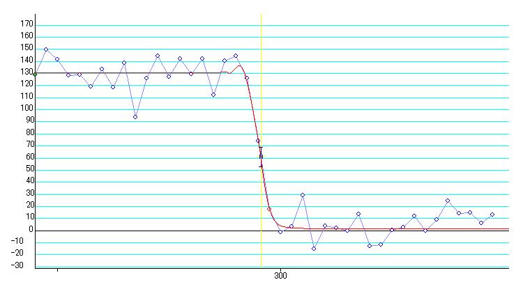
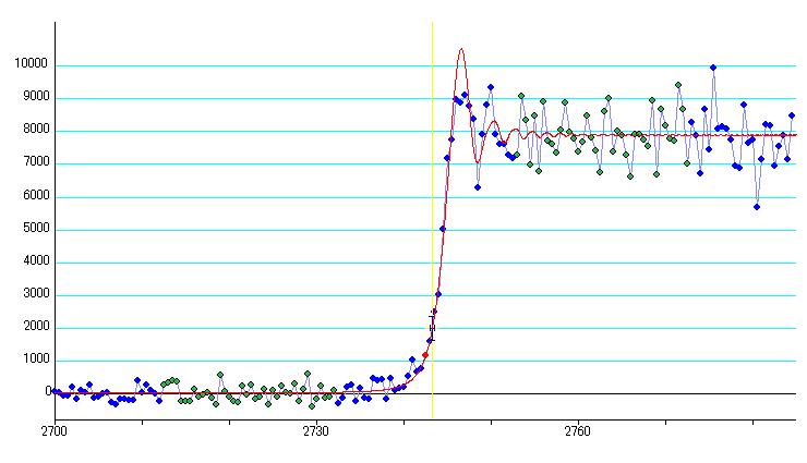
Figure 1. luminous change of XZ4902 fit to star's diameter analysis.

Above figure is luminous change of XZ4902 (pleiades star) occultation in Dec.31 2006. The video has a field which has intermidiate intensity.

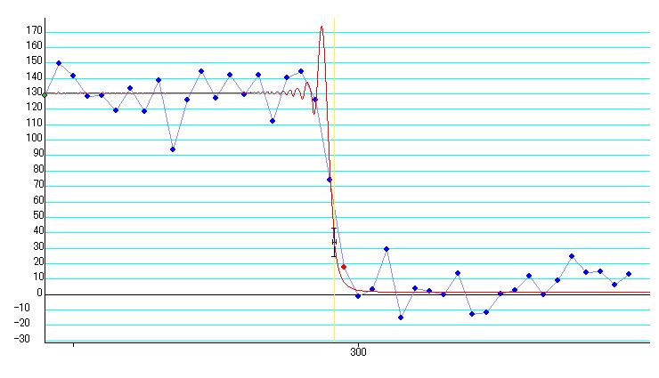
And it is fit to diameter considered simulation. The angular diameter is 18 milliarcseconds. Is this true?

See figure 2.

It seems the light change is different from the light change made from point source simulation. However, the light is integrated during field exposure. Therefore the detail of light curve is “rounded” in the field value. On the other view, the red marked data has possibility that it is not luminous signal but noise, because it is included in the area of background noise.

And also Figure 3 shows the result of double star analysis. It computed 　assuming that two stars whch has same luminous magnitude and 20 milliarcsecond distance from each other. It can be also explained it caused by double star's occultaton.

Figure 1. The result of simulation using point source model.
Parameters for this simulation : Lunar velocity is 814m; lunar distance is 367240km; contact angle is -7degree.
Simulation mode is “for Occultation”.

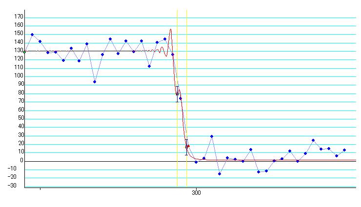
Figure 3. The result of simulation using double model.

This case of analysis shows the cause of gradual event which has only one intermediate point can not been determined to one.